To actually implement a multilayer perceptron learning algorithm, we do not want to hard code the update rules for each weight. Instead, we can formulate both feedforward propagation and backpropagation as a series of matrix multiplies. This is what leads to the impressive performance of neural nets - pushing matrix multiplies to a graphics card allows for massive parallelization and large amounts of data.
This tutorial will cover how to build a matrix-based neural network. It builds heavily off of the theory in Part 4 of this series, so make sure you understand the math there!
Theory
The feedforward step
Consider the following network:
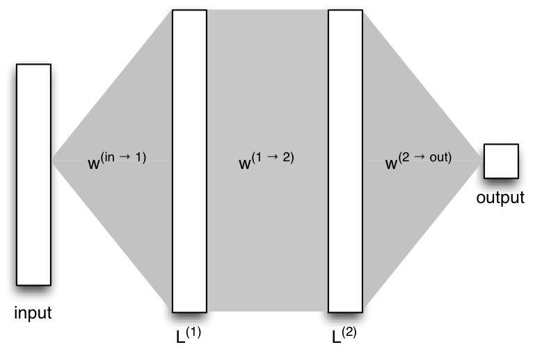
Let's look at the low-level operations needed for the feedforward step as we go from the input $X$ to the first layer $L^{(1)}$. If we want to compute the input for a single unit $j$ in layer $L_1$ for a single example $x$, without using matrices, we would carry out the following operation: \begin{align} s_j^{(1)} =& \sum_{i} x_{i} w^{(in\rightarrow 1)}_{i\rightarrow j} \end{align} That is, for each component $x_{i}$ in the example $x$, we multiply it by the weight that goes from unit $i$ in the input layer to unit $j$ in layer 1. If we want to compute the input to the hidden layer $L^{(2)}$, the only change is that we now include the activation functions of the units in $L^{(1)}$: \begin{align} s_j^{(2)} =& \sum_{i} f^{(1)}(s_i^{(1)}) w^{(1\rightarrow 2)}_{i\rightarrow j}\\ s_j^{(2)} =& \sum_{i} z_i^{(1)} w^{(1\rightarrow 2)}_{i\rightarrow j} \end{align} However, for both of these cases, we must repeat this for every unit $j$ in the layer. In addition, if we have $n$ examples in a minibatch, then we also need to repeat these operations $n$ times, which ultimately leads to a cubic complexity. Nested for loops are generally less efficient than using vectorized code (which can be optimized by handing it off to a BLAS library). A matrix multiply still has cubic complexity, but it is easier to parallelize with a GPU.
Because of this, we will instead formulate our problem as a series of matrix multiplies, where we stuff all of our values into matrices and let the compiler decide how to optimize it. Typically, the rows in our data matrices correspond to items in a minibatch, while columns correspond to a values of these items (such as the value of $s_i$ for all items in the minibatch). Weight matrices have the same number of rows as units in the previous layer, and the same number of columns as units in the next layer.
Consider instead the same network shown above, but with the weights, examples, and unit inputs and outputs all represented in matrix form:

To compute the input activations for $S^{(1)}$ during the feed forward step, we now use the following operation: \begin{align} S^{(1)} =& XW^{(in\rightarrow 1)} \end{align} Let's check the math here. $XW^{(in\rightarrow 1)}$ is an $n\times a$ matrix, so it matches the dimensions of $S^{(1)}$. Based on how we defined our matrices, the value of the element $S^{(1)}_{ij}$ corresponds to the activation of unit $j$ in layer 1 for example $x_i$ in our minibatch. In addition, by the definition of matrix multiplication: \begin{align} S^{(1)}_{ij} =&\ \sum_{k=1}^m X_{ik}W^{(in\rightarrow 1)}_{kj}\\ \end{align} Now if we were to just examine a single row $x$ in $X$ (a single example in our minibatch), we could rewrite this as: \begin{align} S^{(1)}_{ij} =&\ \sum_{i=1}^m x_i W^{(in\rightarrow 1)}_{ij}\\ \end{align} This is equivalent of forward propagation for the non-matrix case: \begin{align} s_j^{(1)} =& \sum_{i} x_{i} w^{(in\rightarrow 1)}_{i\rightarrow j} \end{align} Thus, if we repeat this over all rows in $X$ (i.e. perform a full matrix multiplication), we'll end up with all of the activations for layer 1 for each item in the minibatch. These values are stored in the matrix $S^{(1)}$.
Thus we can propagate the input forward through this network with a series of matrix multiplies: \begin{align} S^{(1)} =&\ XW^{(in\rightarrow 1)}\\ Z^{(1)} =&\ f_1(S^{(1)})\\ S^{(2)} =&\ Z^{(1)}W^{(1\rightarrow 2)}\\ Z^{(2)} =&\ f_2(S^{(2)})\\ \hat{y} =&\ f_{out}\left(Z^{(2)}W^{(2\rightarrow out)}\right) \end{align}
Backpropagation

Again we should check the operations specified in the above schematic to make sure this setup is correct. Recall the general definition of $\delta_j$ for some hidden unit $j$: \begin{align*} \delta_j =& f'_j(s_j)\sum_{k\in\text{outs}(j)}\delta_k w_{j\rightarrow k} \end{align*} Now let's look at how we compute the matrix $D_1$ for the $i$th example in the minibatch (where $\odot$ denotes element-wise multiplication): \begin{align*} D^{(1)} =&\ F'^{(1)}\odot D^{(2)}W^{(1\rightarrow 2)}\\ D^{(1)}_{ij} =&\ F'^{(1)}_{ij}\sum_{k=1}^bD^{(2)}_{ik}W^{(1\rightarrow 2)}_{kj}\\ =&\ f'^{(1)}_{ij}(s^{(1)}_{ij})\sum_{k\in\text{outs}(j)}\delta^{(2)}_{ik}w_{j\rightarrow k}^{(1\rightarrow 2)} \end{align*} We see here that the matrix operations are computing the correct values.
Weight Updates
Algorithm Summary
- Forward propagation:
- Propagate the input to the first layer with $S^{(1)} = XW^{(in\rightarrow 1)}$.
- For each of the hidden layers (that go from index $i$ to $j$) compute $Z^{(i)} = f_i\left(S^{(i)}\right)$ and $S^{(j)} = Z^{(i)}W^{(i\rightarrow j)}$. Store the activation derivatives for the backpropagation step, $F^{(i)} = \left(f'_i(S^{(i)})\right)^T$. Also store $Z^{(i)}$.
- At the output, for the softmax activation function, we have $p(y_i = y) = Z^{(out)}_{iy}$.
- Backpropagation:
- Set $D^{(out)} = (Z^{(out)} - Y)^T$.
- For each of the hidden layers going from index $i$ to $j$, set $D^{(i)} = F^{(i)}\odot W^{(i)}D^{(j)}$.
- Weight updates:
- For the weights going from the input to the output, use $\Delta W^{(in\rightarrow 1)} = -\eta (D^{(1)}X)^T$.
- For the weights leaving a hidden layer $i$ going to layer $j$, use $\Delta W^{(i\rightarrow j)} = -\eta (D^{(j)}Z^{(i)})^T$.
Implementation
In this final section of the series, we'll go over the details on how to implement a fully extensible multilayer perceptron. Formulating the problem as a series of matrix multiplies makes the implementation straightforward - in fact, most of the code here is a direct translation from the theory section. Let's dive in!
Getting the code
You can either check out the latest version of my code from my machine learning Git repository here (the repository is still a bit unorganized), or I've created a stand-alone bundle that you can download here.
The Data
For this tutorial, I'll be using MNIST, which is a standard benchmark in the deep learning community. Most state of the art methods can achieve near-perfect performance on this dataset, so in practice other datasets are used for a fuller comparison, but MNIST is great for a sanity check. We can get pretty good results using a relatively small network.
f = gzip.open('/path/to/mnist.pkl.gz')
train_set, valid_set, test_set = cPickle.load(f)
f.close()

minibatch_size = 100
print "Creating data..."
train_data, train_labels = create_minibatches(train_set[0], train_set[1],
                                              minibatch_size,
                                              create_bit_vector=True)
valid_data, valid_labels = create_minibatches(valid_set[0], valid_set[1],
                                              minibatch_size,
                                              create_bit_vector=True)
print "Done!"
Initializing the network
I have purposefully left out a tunable learning rate, because selecting the proper rate is an art in itself. Instead, I've found a learning rate that works for smaller 2-layer networks. The learning rate does not change during training, nor is there any "momentum," which are both techniques used for more complicated networks.
When we initialized our MLP, we create the input, hidden, and output layers in the file neural_networks.py:
class Layer:
    def __init__(self, size, minibatch_size, is_input=False, is_output=False,
                 activation=f_sigmoid):
        self.is_input = is_input
        self.is_output = is_output

        # Z is the matrix that holds output values
        self.Z = np.zeros((minibatch_size, size[0]))
        # The activation function is an externally defined function (with a
        # derivative) that is stored here
        self.activation = activation

        # W is the outgoing weight matrix for this layer
        self.W = None
        # S is the matrix that holds the inputs to this layer
        self.S = None
        # D is the matrix that holds the deltas for this layer
        self.D = None
        # Fp is the matrix that holds the derivatives of the activation function
        self.Fp = None

        if not is_input:
            self.S = np.zeros((minibatch_size, size[0]))
            self.D = np.zeros((minibatch_size, size[0]))

        if not is_output:
            self.W = np.random.normal(size=size, scale=1E-4)

        if not is_input and not is_output:
            self.Fp = np.zeros((size[0], minibatch_size))
We have some edge cases to consider during this initialization - there are no error signals propagated to the input layer, and the output layer does not have any outgoing weights. Other than that, we initialize our matrices with the proper dimensions according to the algorithm we derived in the theory section. A technique that often helps is to randomly initialize the weights of our network, which we do when initializing the matrix W.
Activation functions
def f_sigmoid(X, deriv=False):
    if not deriv:
        return 1 / (1 + np.exp(-X))
    else:
        return f_sigmoid(X)*(1 - f_sigmoid(X))

def f_softmax(X):
    Z = np.sum(np.exp(X), axis=1)
    Z = Z.reshape(Z.shape[0], 1)
    return np.exp(X) / Z
Note that we do not need to compute the derivative of the softmax function here. In fact, the error signal at the output is still $\delta_o = (\hat{y} - y)$, the same as in the linear case. This is because we use a 1-of-k coding scheme, and we specify a different loss function than in the linear case (if you're interested in more information about this, read the discussion here).Forward propagation
        # We need to be sure to add bias values to the input
        self.layers[0].Z = np.append(data, np.ones((data.shape[0], 1)), axis=1)

        for i in range(self.num_layers-1):
            self.layers[i+1].S = self.layers[i].forward_propagate()
        return self.layers[-1].forward_propagate()
Within the Layer class, we perform the matrix multiply itself:
    def forward_propagate(self):
        if self.is_input:
            return self.Z.dot(self.W)

        self.Z = self.activation(self.S)
        if self.is_output:
            return self.Z
        else:
            # For hidden layers, we add the bias values here
            self.Z = np.append(self.Z, np.ones((self.Z.shape[0], 1)), axis=1)
            self.Fp = self.activation(self.S, deriv=True).T
            return self.Z.dot(self.W)
At the input layer, there is no activation function, so we simply propagate the input data forward through the input layer's weights. If the layer is an output layer, we directly return the value of its output. Otherwise, if we are in a hidden layer, we append a bias weight, compute the activation function derivative, and return the next layer's inputs.Backpropagation
    def backpropagate(self, yhat, labels):
        self.layers[-1].D = (yhat - labels).T
        for i in range(self.num_layers-2, 0, -1):
            # We do not calculate deltas for the bias values
            W_nobias = self.layers[i].W[0:-1, :]

            self.layers[i].D = W_nobias.dot(self.layers[i+1].D) * \
                               self.layers[i].Fp
We first compute the error signal at the output, $\delta_o = (\hat{y} - y)$. We then propagate this error signal backwards through each of the hidden layers.Weight updates
    def update_weights(self, eta):
        for i in range(0, self.num_layers-1):
            W_grad = -eta*(self.layers[i+1].D.dot(self.layers[i].Z)).T
            self.layers[i].W += W_grad
Running the code
Creating data...
Done!
Initializing input layer with size 784.
Initializing hidden layer with size 100.
Initializing hidden layer with size 100.
Initializing output layer with size 10.
Done!
Training for 50 epochs...
[   0]  Training error: 0.57362 Test error: 0.57510
[   1]  Training error: 0.09442 Test error: 0.08670
[   2]  Training error: 0.07088 Test error: 0.06610
[   3]  Training error: 0.04640 Test error: 0.04660
[   4]  Training error: 0.03870 Test error: 0.04260
...
[  46]  Training error: 0.00008 Test error: 0.02670
[  47]  Training error: 0.00006 Test error: 0.02660
[  48]  Training error: 0.00006 Test error: 0.02670
[  49]  Training error: 0.00004 Test error: 0.02690
You can see the training and test error slowly decreasing. Around epoch 50, we begin to severely overfit the training data. However, we're only making about 270 errors on the validation set, which isn't too shabby! To compare, Hinton's landmark dropout paper achieved about 130 errors, beating the previous record of 160 errors. More recent techniques have pushed the rate to well below 100 errors. For such a relatively simple network, we achieve good performance.
Conclusion
I hope this series helped your understanding and gave you a solid foundation to begin understanding more recent deep learning papers. Given enough time, I may write an additional bonus post on some technique used in practice to achieve even better performance (such as dropout, momentum, weight decay, etc.). If you have any questions, please leave a comment!